USUAL DICE EXAMPLE
Imagine that you and I are playing a guessing game. I have two dice, 12-sided and 6-sided, and I am holding them in both of my hands. You are trying to guess which hand has the 12-sided die. At this very moment, there is no information for you. So, it’s not uncommon for a rational agent to think 50-50.
However, you tell me to roll the die I hold on my left hand, and close your eyes. I inform you that I rolled above 3 (i.e., >= 4). Is it still 50-50? It feels like it’s not, since rolling above 3 is more likely with the 12-sided die, right? So, how should you update your initial belief?
I emphasized the “update” above, this is what one should think of when one encounters the word Bayesian: Updating the prior beliefs in the light of new data. Let’s go through the example.
CALCULATIONS
At the beginning, before any information, it’s 50-50: \(P(12\: sided \ LH) = 0.5\) and \(P(12\: sided \ RH) = 0.5\) where LH and RH stands for left-hand and right-hand, respectively. Once you have the information that I rolled bigger than 3, there are two possible scenarios: Either I rolled bigger than 3 with 12-sided or with 6-sided.
- \(P(>3\: |\ 12\ sided) = 0.75\)
- \(P(>3\: |\ 6\ sided) = 0.5\)
Let’s put those in a tree diagram.
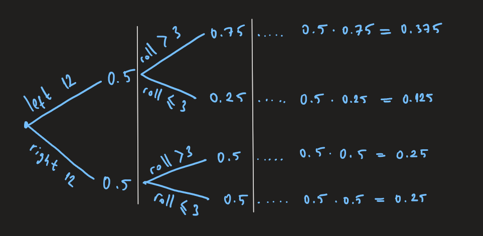
- The first column (left to the first vertical white bar) represents initial beliefs.
- The second column represents the probabilities given the first column.
- Third column is the multiplication of the three, and represents P(A and B).
Well, you are not interested in the whole diagram since you have observed some data: I rolled a number bigger than 3. You wonder:
\(P(12\ sided\ LH\: | >3)\), which is \(\dfrac{P(12\ sided\ LH\: ,\ >3)}{P(>3)}\).
For the numerator, you can track the first row of the tree diagram which leads to 0.375. The denominator consists of two parts, rolling above 3 under two different hypotheses: Following the path of rolling above 3 with 12-sided on the left leads to 0.375, which is the first part. In addition, tracking the other scenario of rolling above 3 with 6-sided on hand leads to 0.25. Hence: \(\dfrac{0.375}{0.375+0.25} = 0.6\)
This represents your new belief of having the 12-sided die on my left hand. If you tell me to roll the die again and construct a new tree diagram, the first column will consist of 0.6 and 0.4 and the following columns would be adjusted accordingly.
DERIVATION
Do you have to construct tree diagram each time? After all, even for this simple question the whole process takes a bit of time. With a little bit of algebra, you don’t have to: \(P(A\: |\ B) = \dfrac{P(A,B)}{P(B)}\). Multiplying both sides by the P(B): \(P(A\: |\ B) P(B) = P(A,B)\) and since P(A,B) = P(B,A)
\(P(A\: |\ B) P(B) = P(B,A)\) which leads to \(P(A\: |\ B) P(B) = P(B\: |\ A) P (A)\)
and voila: \(P(A\: |\ B) = \dfrac{P(B\: |\ A) P(A)}{P(B)}\)
- The left hand side is called posterior probability, and you may come across it in the form of P(hypothesis | data).
- The denominator on the right is total probability of the data, sometimes referred to as marginal probability.
- P(A) is your initial belief here, the prior.
- While P(B | A) is called likelihood which is the probability of the data under given the hypothesis.
For our example: \(P(12\ sided\: |\ > 3) = \dfrac{P(>3\: |\ 12\ sided) P(12\ sided)}{P(>3)}\)
ABOUT THE FRAMEWORK
You may see versions of this where instead of hypothesis there can be theory or parameters (and instead of data, evidence) but they all are the same initially. This type of approach has its advantages such as incorporating the prior knowledge: If I would roll the die again, you would make those calculations with new priors (learned from the first roll), making use of what you already know. It allows for priors that are subjective: Maybe I am known to favor my left hand so it is possible for you to have an initial belief that is not reflected as 50-50.
I will talk more about this view in the future posts but if you’re interested, you can check probability and Bayesian chapter in each of the books below:
- Learning Statistics with R by Daniel Navarro
- Philosophy of Quantitative Methods by Brian D. Haig
- Doing Bayesian Data Analysis by John K. Kruschke
- Improving Your Statistical Inferences by Daniel Lakens
- Think Bayes by Allen B. Downey
and I believe I remember the example above from Mine Çetinkaya-Rundel.